This is one of my favorite projects I worked on while in college! It may not be the neatest, but it shows some of my skills working with Python to clean and prepare data with the Pandas and Numpy packages, as well as use some machine learning capabilities using the sklearn package.

Note : While I had a large hand in this project, this was a collaborative effort between two classmates and myself.

Film Ratings

Stat 426 Final Project

Introduction

Movies are a phenomenon of entertainment that we enjoy on a daily basis. However, not all movies are made equal. There are certain films that reach new heights, while others fall short of our expectations.

One of the metrics we use to rate movies is known as a Metascore. The Metascore is a weighted average of ratings for a movie, which assign more importance to factors like critic reviews and certain publications. This score is supposed to be an objective rating of a film.

We decided that we would look into other forms of data, such as genre of movie, budget, and non-critic reviews to see if we could predict the Metascore of movies.

Data

We are using the “IMDb movies extensive dataset” from kaggle to perform this analysis. This dataset is split into a few CSV files, so we worked to compile the necessary information into a single file for analysis. We performed the proper data cleaning to make sure that it could be used in a model.

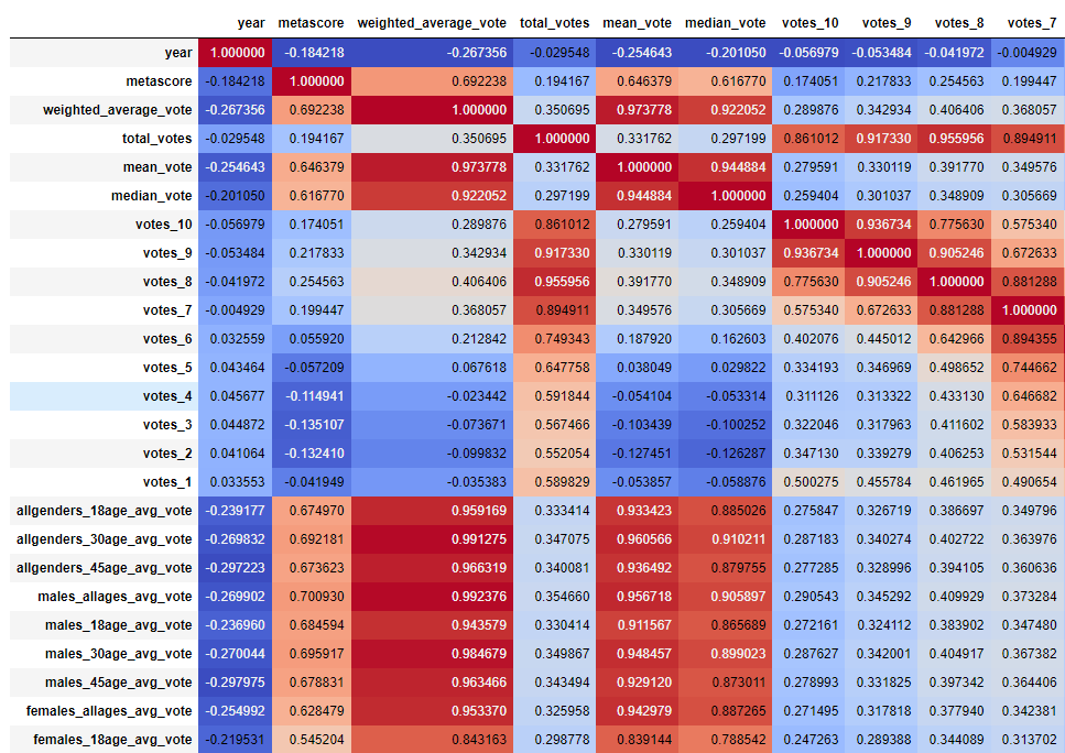
A Correlation plot with the ‘cool warm’ colors showed that there was a high correlation between normal reviews and the Metascore. There are other positive and negative correlations that are weaker but just as interesting, such as Action, Comedy, and Horror movies perform worse than other genres such as Drama and Biography.

(Note : This is only a section of the plot, as the whole plot would be to large to fit here)

data = pd.read_csv('ratings_clean.csv')
corr = data.corr()
corr.syle.background_gradient(cmap='coolwarm')

Corr Plot

Methods and Results

We have all this data, and we have processed it using pipelines. We want to be able to predict the Metascore with all the other variables. to do this we will fit the data to 4 types of models.

Lasso Regression
K Nearest Neighbors Regression
Linear Regression
Decision Tree Regression

laspipe = Pipeline(steps=[('preprocessor', preprocessor),
                      ('regressor',  Lasso(alpha=.5))])

knnpipe = Pipeline(steps=[('preprocessor', preprocessor),
                      ('knn',  KNeighborsRegressor(n_neighbors=5))])

lrpipe = Pipeline(steps=[('preprocessor', preprocessor),
                      ('linearregression', LinearRegression(fit_intercept=False))])

dtpipe = Pipeline(steps=[('preprocessor', preprocessor),
                      ('decisiontreeregressor', DecisionTreeRegressor())])

At this point we have the models fitted with the appropriate data, and now we have to test to see how well they do. We can use a few metrics to test, and today we will be finding the cross validation scores for the Mean Square Error (MSE), Mean Absolute Error (MAE), and Root Mean Squared Error (RMSE).

# Cross Validation score for Mean Absolute Error

# lasso
MAE_las = cross_val_score(laspipe, X_train, y_train, scoring='neg_mean_absolute_error')
print(np.mean(MAE_las)*-1)

9.954055146050106

# knn
MAE_knn = cross_val_score(knnpipe, X_train, y_train, scoring='neg_mean_absolute_error')
print(np.mean(MAE_knn)*-1)

10.110086327556242

# linear regression
MAE_lr = cross_val_score(lrpipe, X_train, y_train, scoring='neg_mean_absolute_error')
print(np.mean(MAE_lr)*-1)

55.94360681218829

# decision trees
MAE_dt = cross_val_score(dtpipe, X_train, y_train, scoring='neg_mean_absolute_error')
print(np.mean(MAE_dt)*-1)

12.220234259501556

Based on this metric of Mean Absolute Error, Lasso is closest with an average error of only 9.9, as opposed to Linear Regression, which has an average error much higher.

# Cross Validation score for Mean Squared Error

# lasso
MSE_las = cross_val_score(laspipe, X_train, y_train, scoring='neg_mean_squared_error')
print(np.mean(MSE_las)*-1)

154.0117768943061

# knn
MSE_knn = cross_val_score(knnpipe, X_train, y_train, scoring='neg_mean_squared_error')
print(np.mean(MSE_knn)*-1)

162.22024677361998

# linear regression
MSE_lr = cross_val_score(lrpipe, X_train, y_train, scoring='neg_mean_squared_error')
print(np.mean(MSE_lr)*-1)

3274.046691663391

# decision trees
MSE_dt = cross_val_score(dtpipe, X_train, y_train, scoring='neg_mean_squared_error')
print(np.mean(MSE_dt)*-1)

240.77650113730147

Here we have Lasso performing the best with a mean squared error of around 154.

# Cross Validation score for Root Mean Squared Error

# lasso
RMSE_las = cross_val_score(laspipe, X_train, y_train, scoring='neg_root_mean_squared_error')
print(np.mean(RMSE_las)*-1)

12.409150667849222

# knn
RMSE_knn = cross_val_score(knnpipe, X_train, y_train, scoring='neg_root_mean_squared_error')
print(np.mean(RMSE_knn)*-1)

12.735243529891704

# linear regression
RMSE_lr = cross_val_score(lrpipe, X_train, y_train, scoring='neg_root_mean_squared_error')
print(np.mean(RMSE_lr)*-1)

57.21908102086684

# decision trees
RMSE_dt = cross_val_score(dtpipe, X_train, y_train, scoring='neg_root_mean_squared_error')
print(np.mean(RMSE_dt)*-1)

15.600191607587442

And finally the Root mean squared error shows to us for the third time that Lasso Regression is the best for this data.

We can see that Linear Regression is the worst at predicting, with much higher error rates than the others. The Lasso model is much more accurate for this job. regardless, lets predict the scores using test data.

yhat_las = laspipe.predict(X_test)

# knn
yhat_knn = knnpipe.predict(X_test)

# linear regression
yhat_lr = lrpipe.predict(X_test)

# decision trees
yhat_dt = dtpipe.predict(X_test)

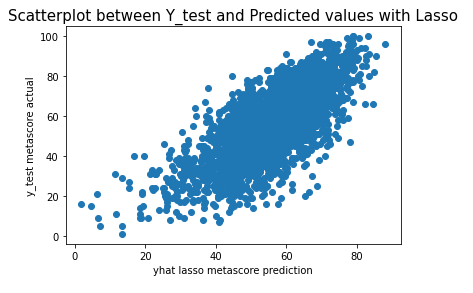
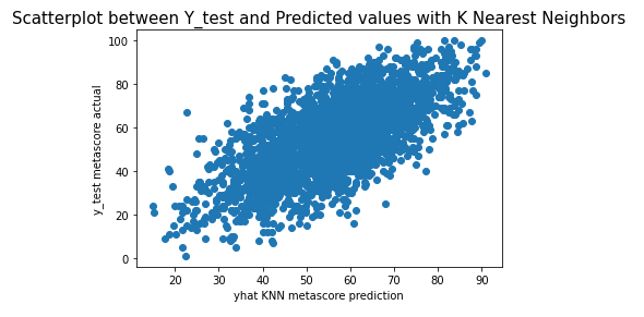
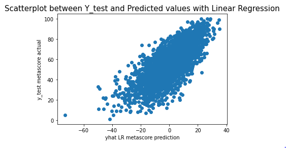
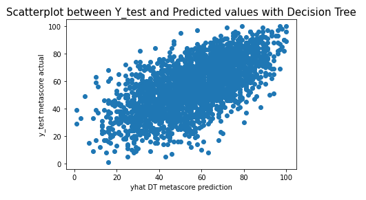
We now have an array of predictions for a Metascore. Lets visualize our data to see how well we did!

plt.scatter(yhat_las, y_test['metascore'])
plt.xlabel("yhat lasso metascore prediction")
plt.ylabel("y_test metascore actual")
plt.title("Scatterplot between Y_test and Predicted values with Lasso", fontsize=15)

Lasso Plot

plt.scatter(yhat_knn, y_test['metascore'])
plt.xlabel("yhat KNN metascore prediction")
plt.ylabel("y_test metascore actual")
plt.title("Scatterplot between Y_test and Predicted values with K Nearest Neighbors", fontsize=15)

KNN Plot

plt.scatter(yhat_lr, y_test['metascore'])
plt.xlabel("yhat LR metascore prediction")
plt.ylabel("y_test metascore actual")
plt.title("Scatterplot between Y_test and Predicted values with Linear Regression", fontsize=15)

Lasso Plot

plt.scatter(yhat_dt, y_test['metascore'])
plt.xlabel("yhat DT metascore prediction")
plt.ylabel("y_test metascore actual")
plt.title("Scatterplot between Y_test and Predicted values with Decision Tree", fontsize=15)

Lasso Plot

Conclusion

In all of the models, we were able to make a close prediction. the Linear Regression model was the weakest relationship of the bunch, And the Lasso model performed much better.

We did not have the capability to test all factors though. In future analysis, we would hope to include important features such as Actors, Directors, and Screenwriters to better predict how a movie will perform critically.